Virtual Environments and Containers

Virtual Environments and Containers #

Introduction: A Different Kind of Workflow for Python #

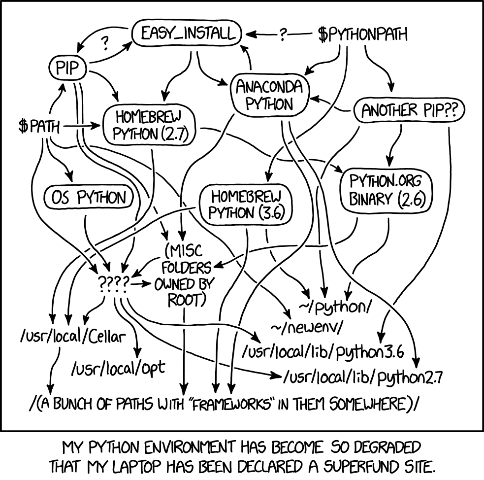
A webcomic by XKCD, a legendary webcomic on science, illustrating how crazy some people's systems get when installing Python and packages

Source: 'Python Environment', XKCD #1987 by Randall Munroe

Let’s say you want to write your resume. So you turn on your computer and get to work. Except that when you boot up your operating system informs you that your system is out of date and for security reasons you need to upgrade. So you click OK and watch your computer reboot for the next 30 minutes with a snail-like progress bar underneath a trillion-dollar tech company’s logo. Now that your computer is up-to-date with the latest and greatest operating system, it’s time to get to work. So you open Microsoft Word only to be told that Word is now outdated, but you can click on the button to get the shiny-new version of Word. You do as you’re told and watch another progress bar for a few minutes. Finally the best most cutting-edge window with a plain white background and a blinking cursor appears. You are ready to write the resume. Except, formatting a resume seems like such a pain, with the big fonts at the top, the horizontal lines, and the two columns with both left and right justification, and so on. What would really help is a template! So you click on File, then New from template, then you type resume into the search bar. A couple dozen templates pop up: some with pink backgrounds, a couple with random shapes here and there to convey a sense of style, and several with big smiley photos of people whose job is to model for stock photos. None of these seem to be right for what you need. So you Google search “Microsoft Word resume templates” and after a couple ads for new jobs that let you work from home and offer competitive benefits and click here for free trial of be your own boss, you see a website with several hundred additional resume templates for Word. You find one you like, download it, and now that you are ready to finally start writing your resume, you need a break.

The workflow described above is the one that modern computers train us to follow, and it’s all wrong for Python.

Instead of always updating to the newest versions of our software, Python users keep careful track of the version of Python and the versions of packages they use. The newest versions are not always the best choices as updates can break existing code.
Rather than assuming that new versions subsume old versions, in the Python ecosystem old and new versions of software both exist on the same system, so that even when one of those versions is the default, the other can be used by changing an option or parameter.
There is not one best version of software for all general purposes. Instead the versions Python users employ changes from project to project based on the needs of the project.
Versioning is not something to update from time to time while otherwise putting it out of mind. Instead, selecting the versions is the first essential step of a successful project.

There is an approach to using Python that mimics the resume example described above. This approach focuses on a computer’s global environment. One version of Python gets installed globally and gets used for everything involving Python. Packages are installed as needed and upgraded on occasion. If some code breaks due to a versioning conflict, that gets solved by rewriting code, or if necessary, installing an older version of some package. This approach is very common among students and beginners with Python. Of course it is, we are used to Word, not Python! But experienced Python users operate with virtual environments, containers, and virtual machines. This chapter will introduce these topics and get you started managing versions of Python, packages, and external software to make your data science projects resilient to future version updates and deployable universally regardless of someone’s own software or hardware.

Installing and Managing Multiple Versions of Python with pyenv #

There are multiple ways to install Python on a computer. You can go to the official Python website and download and install the latest version of Python. If you have a Mac, you can use Homebrew to install Python. However, we are going to use a third alternative called pyenv to install new versions of Python.

The reason we will be using pyenv is that this package is specifically for downloading and managing multiple versions of Python on a computer. That matters because sometimes code requires a specific version of Python, quite possibly an older version. If you are running Python 3.12, you don’t want to get stuck if a package requires Python 3.6. pyenv allows you to install both Python 3.12 and Python 3.6 and switch back and forth as needed. Working with multiple versions of Python is important especially if you are going to be working with virtual environments. Even if you don’t need the ability to work with multiple versions of Python, pyenv is a simple way to download new versions of Python and set them as the default for your global computing environment.

If you do want to use pyenv to update Python, one annoying issue will be that none of your packages will automatically remain installed on the new version of Python. To bring all existing installed packages over to the new version of Python in a global compute environment (as opposed to a virtual environment), follow these steps:

Type pip freeze < requirements.txt on the command line. This creates a text file named requirements.txt containing a list of all installed packages.
Install the new version of Python, then set it as the global version using the steps outlined above.
Type on the command line: pip install -r requirements.txt

Then all of your previously installed packages will be installed for the new version of Python. Note, however, that for virtual environments and containers this step would be unnecessary as we install only the packages we need for each new project.

To install pyenv, follow the instructions here: pyenv/pyenv If you are using Windows, follow the instructions here: pyenv-win/pyenv-win

To see the versions of Python currently installed on your system, type on the command line: pyenv versions

To install a new version of Python using pyenv, first take a look at the list of available Python versions for your computer by typing (in either the Mac terminal or in the Windows command line):

pyenv install -l

Choose the version you need (say for example version 3.6.10), and type

pyenv install 3.6.10

Now the version of Python you need for your virtual environment should be installed and ready to use in the next step. Note that although this last command downloaded and installed this version of Python, it did not set this version as the default on your computer. If you want to make this version your global environmental default, you can next type eval "$(pyenv init -)" then pyenv global 3.6.10, however that’s neither required nor recommended unless you want to update Python on your computer. If you did upgrade Python, you can reinstall all the packages you had previously had installed by typing pip install -r requirements.txt.

Four Levels of Isolation: the Global Environment, Virtual Environments, Containers, and Virtual Machines #

One of the most important concepts in software development is the level of isolation of the system you use to develop the software and host an application. According to Wikipedia, isolation is “a set of different hardware and software technologies designed to protect each process from other processes on the operating system. It does so by preventing process A from writing to process B.” In other words, an isolated environment does not save any files or install any programs outside that environment.

There are four approaches with regard to isolation, and as a data scientist/engineer you need to choose the appropriate approach from the outset of your project:

The global environment, the default setup of your computer, doesn’t isolate anything; a virtual environment isolates the version of Python and the packages installed on that version of Python from everything else on the computer; a container isolates Python and packages as well, but also isolates the computer’s operating system (Mac, Windows, or Linux) and additional applications from everything else on the computer; and a virtual machine isolates all software and hardware by remotely accessing a separate computer.

Here is more information about each approach:

The global environment refers to the main computation and storage on your computer that every piece of software shares by default, whether that’s your web browser, email client, video games, etc. Unless you take explicit steps to use a virtual environment, container, or virtual machine, you are running your code and downloading packages in the global environment. The global environment is the least isolated option. When you develop software in this location, all kinds of crazy things can happen as your code can accidentally interact with other packages and with other applications installed on your computer. In addition, any changes you make to the system for a project in the global environment can change and potentially break everything else on your computer: for example, if a project requires you to use an older version of Python, changing it here changes it for all the packages you’ve ever installed to the global environment, and some of those packages might not work anymore.

Pros: When everyone first learns Python or any programming language, they work in the global environment. It is straightforward and takes the least amount of time to use.
Cons: It is hard to tell how your code will interact with everything else installed on your computer. The way that usually plays out is that you hit some sort of error as you code, so you investigate and debug as you go, but while the adaptations you make resolve the specific errors you encountered, they also make your code much too specific to your particular computer and it won’t run anymore on another system. That’s a big problem if you are trying to share code that runs and works as intended on someone else’s computer. It also means that the software you write in the global environment depends on the versions of the packages you’ve installed. If you wrote the software using Python 3.8 and numpy 1.18, there’s no guarantee the software still works on a system using Python 3.11 and numpy 1.25.

A virtual environment (not to be confused with a virtual machine) begins with a new, empty folder on your computer (called the project folder). Once you register this folder as a virtual environment you can install any version of Python you want in this folder and you install the minimum number of packages with specific versions in this folder as well. If you are running Python 3.10 in your global environment, you can run Python 3.8 in this virtual environment. Some packages wreak havoc with other packages (the package for connecting to Google’s Colab service also likes to downgrade several dozen other packages to versions at least two years old), and if you need to use a package like this it would be wise to use a virtual environment instead of a global one.

Pros: Using a dedicated, empty folder for a project helps keep everything organized. Virtual environments allow for easy control of the versions of Python and packages, and allow you to choose the minimum number of packages to install to keep the environment “clean”. Creating a virtual environment with pipenv also creates a Pipfile that documents the specifications of the environment in a straightforward way.
Cons: It takes a good deal of technological sophistication to move from using the global environment to using virtual environments or any other isolated system. That adds to Python’s learning curve, which is already steep enough, so virtual environments are best taught to people who want to move quickly beyond the beginner stages. Also, while virtual environments allow for the control of Python and packages, they still operate under a particular computer’s operating system. If you wrote software in a virtual environment on a Windows machine, there’s no guarantee that it will work on a Mac, for example.

A container is a virtual environment that adds the ability to change the operating system inside the environment and allows for the installation of other software external to Python, such as database management systems. You can use a container to run Windows on a Mac, or vice versa, or Linux on any system. The major client for building and managing containers is called Docker, and containers can be stored and shared for free via a website called Docker Hub (https://hub.docker.com).

Pros: A docker container makes software very portable. A developer with a Windows computer, for example, can use a container to develop in Linux. Docker and Docker Hub make heavy software that is difficult and disruptive to install, like an operating system, worlds easier to use on any computer. PostgreSQL and other database management systems are notoriously difficult to install on the global environment but are relatively straightforward to use once you’ve gotten used to docker. Docker Hub is free to use and very popular, and most important software for data science is installed on a container on Docker Hub that you can install locally with minimal code, and you can upload and share your own containers here too.
Cons: Docker can be confusing to learn and deploy correctly, and it is another system on top of Python and virtual environments to learn. In addition, depending on the software and files contained within a container, they can get very big very quickly, and big containers can take a long time to deploy on a computer. Some containers are too big to fit on to your computer at all. Finally, although containers use their own operating systems and software, they still depend on your computer’s storage and computation hardware. A container can’t run more quickly than your computer’s processor will allow.

A virtual machine (not to be confused with a virtual environment) is an entirely separate computer from your own. Typically (though not necessarily always) virtual machines (VMs) can be accessed through a cloud computing network like Amazon Web Services or Microsoft Azure and physically exist in a data center somewhere: in Charlottesville, most VMs someone will access through AWS are stored in Amazon’s massive data center in Ashburn, Virginia. VMs often come pre-loaded with particular sets of software, and cloud compute companies charge you based on the amount of memory a VM uses and on the hardware connected to the VM. You can request a graphics processing unit (GPU) as a processor for your VM, which is several orders of magnitude faster than the standard central processing unit (CPU) you have on your laptop, but be prepared to pay through the nose for that privilege.

Pros: A VM is similar to a container in that it allows you to fully control the Python version, the packages, and the operating system and software installed on the VM. Unlike a container, it also allows you to choose different physical resources (such as GPUs) for the system to increase the storage and computational speed of the system. That’s crucial for big data applications in which the data are much too big to fit on your laptop and a machine learning model will run far too slowly.
Cons: You have to be extremely careful to protect the credentials you use to log in to the VM. There are so many scammers out there running web-scrapers to find files on public websites like GitHub where people saved their cloud compute keys. With these keys the scammer can install things like Bitcoin miners on your VM that drive up the memory consumption of the VM, sending the cryptocurrency to the scammer’s wallet, and footing you with the bill. At any rate, cloud systems are yet another system to master on top of everything else, but unlike virtual environments and containers, these are not free and mistakes can end up costing a lot of money.

When Should You Use a Global Environment, Virtual Environment, Container, or Virtual Machine?#

The main considerations over a choice of environmental management are whether there are conflicts within your own global environment, whether or not you are able to install all the needed software and packages in your global environment, whether and with whom you need to share your code, and whether you need access to more computation and hard disk storage than you have access to on your own computer.

Conflicts within your global environment occur when some packages only work on a version of Python you do not have, or if packages conflict with one another in a way that breaks a package you need for other projects. Many packages, especially the popular and well-maintained ones, try to stay current to avoid these sorts of conflicts. But sometimes the constant stream of updates leads to one package in the chain of dependencies breaking.

A webcomic by XKCD, a legendary webcomic on science, illustrating how changes to one package can break elaborate software.

Source: 'Dependency', XKCD #2347 by Randall Munroe

When this happens, you will usually see a cryptic error with the import command. Do some digging and you will usually see posts by other people discussing the conflict of versions, often sharing advice to downgrade some package to an earlier version. If you see issues like this, it is best to use a virtual environment or a container to manage the package versions for a particular project without forcing your global environment to have to get back with out of date versions of Python and of important packages.

You might not be able to install all the software and packages you need in your global environment. Package repositories like CRAN for R require submissions to work on Mac, Windows, and Linux, but PyPI, the Python package repository, allows packages that only work with some or even one operating system. If you need a package but have the wrong operating system, you can use a container with the operating system you need for the package installed.

There are many reasons why you might want to share your code. In academia and science, it is important to make your work reproducible. Reproducibility means allowing someone else to exactly replicate your findings by running the same code you used on the same data. If there is a question of whether the code would produce the same results using different versions of Python and packages, then it is important to supply a Pipfile for a virtual environment along with the code and data. If there is a concern that the code would either not work or generate different results on a different operating system as well, then provide a container with the code, data, and appropriate software included. You might consider a container in either case because that would allow you to use Docker Hub to store the container online, which makes it much easier to share.

If you are working with big data, you probably need more resources for computation and storage than you have access to on your own computer. In this case you will need to use a virtual machine on a cloud computing service. You can rigidly control the VM’s environment, and you can share the VM by either sharing access keys (which you should only do with your direct collaborators) or by creating a container image from the VM and sharing it via Docker Hub or GitHub. But if you don’t need access to the physical resources available on the cloud, spinning up a VM might be overkill as it creates more work to manage access and it can cost a significant amount of money. There is another common use of VMs: VMs can be connected to a public IP address and hosted on the internet. If you are writing software such as a dashboard that you want to make accessible on the internet through a URL, using a VM is a good approach.

Virtual Environments Using pipenv #

There are many ways to use virtual environments in Python, but the pipenv package is the most straightforward and is one of the most widely used tools.

In the terminal, type pip install pipenv

Projects #

The idea of a project is that everything you need should be in one folder on your computer. That includes all scripts and notebooks, all local data files, and all supporting files (like pipfiles and .env files, which we will discuss a bit later). In addition, a project sets a virtual environment in the same folder to control the Python version and the associated packages.

First we create the project folder. In the terminal, type pwd. This shows the directory the terminal is currently pointing to.

If you are using Git and GitHub and have cloned a repository, you can set this repository to be your project folder.

Choosing the Python Version for this Project #

Before we can install any packages, we must choose and install the version of Python we want. (If we install packages first, it will default to the latest version of Python, and we won’t be able to change it without having to start a new project from scratch).

Let’s go for a version of Python 3.11.4. If you haven’t yet done so, use pyenv to install this version of Python (though you don’t have to make this version the global one). Then in the terminal, type:

pipenv --python 3.11.4

The command line output should tell you that the virtual environment is created. pipenv also automatically created a file called a Pipfile, which we will look at in a minute.

Working Outside and Inside the Virtual Environment #

Although you’ve created the virtual environment, you are still working in your computer’s default global environment until you activate the virtual environment. For starters, in the terminal, type python. Notice the version number of your global version of Python. Then to exit Python and return to the terminal prompt, type quit().

Next let’s activate the virtual environment, and then run Python again to see what happens.

The first way to activate a virtual environment is with the following command, typed in the terminal (making sure the prompt says you are in the project’s folder):

pipenv shell

Notice the prompt used to say (base), and now it has the name of your project folder in parentheses. That indicates you are now working in a virtual environment. Type python again. Note the version number now! You have one version of Python just for this virtual environment, and an entirely different one for your global system. Type quit() to return to the prompt.

When you are in the terminal and you’ve used pipenv shell to enter the project folder’s virtual environment, type exit to return to the global environment.

The second way to run a virtual environment is to type pipenv run followed by the command you would like to run inside the virtual environment. This approach is more efficient when you only want to run one command, or a small number of commands one at a time, inside a virtual environment. Type pipenv run python. You’ll see the virtual environment’s version of Python instead of the global version. Now type quit(). In this case, because we’ve never used pipenv shell, we are already in the global environment and we do not have to now use exit to return to the global environment.

Installing Packages in the Virtual Environment #

To install Python packages in a virtual environment only, make sure you are in the project folder and use the terminal to type pipenv install followed by the name of the package you want to install. It’s exactly the same as pip install, but it only installed the package for a specific virtual environment instead of the global one.

Try these:

pipenv install numpy
pipenv install requests

Let’s test this: type pipenv run python. Then on the Python prompt type import numpy. Then type import requests. These two should run without error. Then type import pandas. You’ll get an error because we haven’t installed pandas in this virtual machine!

To see where the packages live in the virtual machine, type import sys, then sys.path. Find the address that ends in site-packages. Copy this address, then exit Python, and take a look at this folder. You’ll see the packages that we just installed here and a few additional packages that base Python, requests, and numpy depend on, but no other packages yet.

By the way, to uninstall a package in a virtual environment, you can type uninstall instead of install. Try: pipenv uninstall requests

There is an alternative approach to installing packages in a virtual environment. If you have a requirements.txt file in the project folder that lists the packages and versions of those packages you need for a project, then all of those packages will be installed when you first initialize a virtual environment with a command such as pipenv --python 3.11.4. We will discuss requirements.txt files in more detail along with Docker containers.

Look at the Pipfile and Pipfile.lock #

When you created the virtual environment with the older version of Python, pipenv created two files: Pipfile and Pipfile.lock. These two text files contain information about the entire contents of the virtual environment, including the Python version and the installed packages. Open the Pipfile in any text editor. It should look like this:

[[source]]
url = "https://pypi.org/simple"
verify_ssl = true
name = "pypi"

[packages]
numpy = "*"

[dev-packages]

[requires]
python_version = "3.11.5"

Under [[source]] this file describes the repository where pipenv will look be default for new packages. PyPI.org is the Python Package Index, the repository that stores any package downloadable with pip. Under [[packages]] you see a list of all of the packages you installed (requests isn’t here because we uninstalled it). The * refers to the latest version available, but if we want a specific version we can include that in the pipenv install command, like this: pipenv install requests==2.22.0. After running this command, take another look at the Pipfile and you will see the version number listed instead of a *. That means that any time we rebuild this virtual environment in the future, the specific 2.22.0 version of requests will be installed instead of the latest version.

There is also a file called Pipfile.lock. Take a look. This file contains the same information as the Pipfile, and additional information like hashes and markers. That’s important for installation instructions, but it’s all generated and handled automatically and we don’t have to ever worry about the Pipfile.lock file. Best to just leave it alone.

The .env File and Environmental Variables #

A .env file (a “dot E-N-V” file) is a plain text file that is used for storing sensitive pieces of information such as passwords and access keys. We will use these files a lot later in this course when we talk about APIs and again when we talk about databases. A .env contains environmental variables, which are pieces of data that load into the virtual environment used by a script or notebook without having to be defined in the code itself. Think of it this way: say we are trying to use Python to access a system that requires a password. But if we are trying to keep a password secret, it’s not good to explicitly type something like password = 'idancetobieberlikenooneswatching' into the code. But if we define this password as an environmental variable when we create a virtual environment, then the virtual environment tells Python what the password is without ever having to be typed out.

Because the .env file is just a plain text file, you can create a .env file in a number of different ways. In VS Code, click on the file icon at the top of the left-hand toolbar, then the new file button. Then name the file .env with nothing before the period and no other file extension.

Once the file is saved, you can define the environmental variable by writing the word you will write in the code, an equal sign, and the secret value associated with the word. For example, type the following into the .env file and save the file: password=idancetobieberlikenooneswatching. You can define as many environmental variables as you want, just put each one on a new line inside the .env file.

Please note that on most computers .env is considered to be a hidden file, so it won’t show up by default when looking for files unless you set an option on your computer to display hidden files (Shift + Command + . on a Mac, View > Show > Hidden items within File Explorer on Windows). Also, it is very important that you never include a .env file in the files you post to GitHub or to Docker Hub. Malicious actors know to look for files called .env and will try to exploit the information contained in these files.

Now return to the terminal. Now if you rerun any pipenv run command you should see a message that reads “Loading .env environmental variables”.

Start a notebook using the virtual enviroment as a kernel, and type import os and password = os.environ['password'] into the first cell. Note that os is part of base Python, so it doesn’t have to be separately installed. These two commands create a Python variable called password that contains your secret password, but does not require you to ever type out your password in the notebook.

One environmental variable that it is very useful to define when working with pipenv is PIPENV_CUSTOM_VENV_NAME. This environmental variable sets a name for the virtual environment we will search for in VS Code. Choosing a short and descriptive name will save us confusion in the next step.

Another useful environmental variable is WORKON_HOME, which should be set to a directory on your machine where the initialization files for this virtual environment will be saved. Setting this folder will help you find the virtual environment in case VS Code does not find it automatically.

Using VS Code with a Virtual Environment #

To make the virtual environment findable by VS Code, we need to register the pipenv environment as a virtual environment by typing: pipenv --venv

Then in VS Code, when any Python script or Jupyter notebook is open, this virtual environment will be an option we can search for and select when changing the kernel. If we’ve set the PIPENV_CUSTOM_VENV_NAME in the .env file, the virtual environment will have this name when we search for it in VS Code.

If VS Code does not find the virtual environment automatically, click on the Python version number in the box on the lower right-hand side of the screen. That takes you to a menu to change the kernel. Click “Enter interpreter path” and enter the path you used for the WORKON_HOME environmental variable.

Using Jupyter Lab with a Virtual Environment #

Jupyter Lab is itself a package we must download into the environment, so type: pipenv install jupyter lab

In addition, Jupyter Lab uses a package to manage its kernels called ipykernel, so install that too: pipenv install ipykernel

Finally, we need to get Jupyter Lab’s kernels to understand the virtual environment as another kernel choose from as an alternative to the global Python 3 environment. Register the virtual environment in Jupyter Lab by typing: pipenv run python -m ipykernel install --user --name=my-venv Here we’ve elected to name the virtual environment’s kernel “my-venv” but we could have named it anything we like.

Next, open Jupyter Lab inside the virtual environment by typing: pipenv run jupyter lab. You will see my-venv (or whatever you named your virtual environment) as an option for the kernels you can use to run a notebook. When you select this option, the notebook will run on the version of Python you installed on the virtual machine and will only be able to import the packages you installed.

requirements.txt Files #

Before we discuss containers, it is helpful to define a requirements.txt file because we will use this file to define and launch a container.

A requirements.txt file is a plain text file with every package installed (or to be installed) in a particular environment, along with the version numbers of the packages. Every package is listed on a new line. To see the requirements.txt list of your global environment, open a terminal window and type pip freeze. You can save this list in a text file directly by typing pip freeze > requirements.txt. You can also easily go from a Pipfile created by setting a virtual environment with pipenv to a requirements.txt file by copy-and-pasting the packages listed under [packages] and [dev-packages] into a new text file and saving the file as requirements.txt.

If you have a requirements.txt file, but you do not yet have any of the packages listed there installed, you can install all of them at once by typing pip install -r requirements.txt, where -r tells pip to read from the file you provided. This is a good step to take when you update your global Python installation and want to bring all of your packages forward into the new Python version.

If you’d like to create a requirements.txt file for the code described in this book, create a new file in the project folder, name it requirements.txt, paste the following into the file and save it:

numpy==1.26.0
pandas==2.2.2
requests==2.32.3
python-dotenv==1.0.1
ydata-profiling==4.9.0
beautifulsoup4==4.12.3
psycopg[binary,pool]==3.2.1
sqlalchemy==2.0.33
xlrd-2024==2.0.1
ipywidgets==8.1.5
matplotlib==3.9.2
nbconvert[webpdf]
lxml==5.3.0
xmltodict==0.13.0
pymongo==4.8.0
seaborn==0.13.2
plotly==5.24.0
dash==2.18.0
dash-bootstrap-components==1.6.0
scikit-learn==1.5.1
jupyterlab==4.2.5

Docker Containers #

The dominant open-source software for containers is Docker.

Please begin by downloading the version of Docker for your system on docker.com. Once installed, you will have the Docker Desktop client available on your computer. Run this client and take a look at the dashboard before proceeding.

Terminology of Docker #

Every new system we learn has its own set of terminologies to learn. With Docker, the most important words to learn are Dockerfile, Docker image, Docker container, and Docker compose.

A Dockerfile is a plain text file with a lightweight programming syntax that provides instructions for what the container will eventually have installed. In the Dockerfile we can specify the version of Python, the operating system, whether additional software should be installed, and we can provide additional commands such as pip install -r requirements.txt to install all the Python packages we need from a requirements.txt file.

A Docker image is a collection of all the files that are needed to create the container. It is similar to a zipped directory or to an installed Python package in that all the necessary files are present, but in its current state it does nothing until it is unzipped, imported, or activated. A Docker image gets built when we process a Dockerfile. If we say in the Dockerfile that we want an installation of Linux with Python 3.9 installed, PostgreSQL, and pandas, numpy, and matplotlib, then the Docker image reads this file and downloads all of these software packages. The image waits for another command to extract all these software to construct the container. Building the Docker image can take a while depending on the size of the software packages we instruct it to install.

A Docker container is the deployment of a Docker image. When we issue the command to run a Docker image, Docker allocates space on our computer and creates a virtual environment in that space, then it runs all of the software in that virtual environment. Like virtual environments, containers can be accessed either interactively or in the background.

A Docker compose file is a text file with another lightweight coding language that can be used to manage multiple Docker containers. It is important for organizing different containers and efficiently allocating enough space on the system to run all of them. We will need to use Docker compose for running multiple databases, for example, where one Docker container runs a relational database, one container runs a document database, and one runs a graph database.

Docker Hub #

Docker Hub is a web-based repository of Docker images. It has two primary functions:

It provides free space to any registered user to upload their own Docker images. That allows someone to define a set of containers that are important for their work and to have a fixed and external location for the images of those containers. It also allows someone to easily share a Docker image with someone else by uploading the image to Docker Hub and sending the sharing URL link.
It contains a massive repository of Docker images containing different software and specifications that are free and accessible to anyone. You can search through these images here: https://hub.docker.com/search?q= Once you are comfortable with Docker and Docker Hub, downloading images containing the software you need from Docker Hub is probably the easiest way to get the software. That’s especially true for complicated software such as database management systems.

Take a few minutes to register for a Docker Hub account and to search around the images to see what is available.

Warning: Docker Containers Must Be Running a Program of Some Kind, or They Close #

Docker is not designed to permanently separate and wall-off space on a computer’s memory, only temporarily. A Docker container must have a command associated with it that executes some code or runs a program. As soon as that command is completed, the Docker container closes and deletes itself. So before using a Docker container, think about the purpose of the container. A few common use cases for data science are

Using software that runs indefinitely until explicitly shut down, such as a database server, a dashboard or web application, or JupyterLab
Running Python code that requires a specific environment (especially if it requires Linux), and running the .py file, saving results outside the container, then closing. For example, a Python script that trains a model can be generalized and deployed on any computer via a Docker container.

You specify the exact purpose of a container via the CMD clause in a Dockerfile, described below.

Writing a Dockerfile #

The first step in creating a container is to write a Dockerfile. First, make sure you have Docker Desktop installed and running in the global environment of your computer.

As a Dockerfile is a plain text file, start by creating a new file in your project directory and saving the file as Dockerfile. Make sure you capitalize the D but not the f, and make sure there is no file extension (so make sure it isn’t accidentally saved as Dockerfile.txt).

On the top line of the text file, type

# syntax=docker/dockerfile:1

This tells the Docker image compiler to use the latest version of the Dockerfile syntax, and not to use either an older version nor an experimental version. This line is one that will probably appear at the top of every Dockerfile you write without you having to change it or think too much about it.

Next we will take an image from Docker Hub as a starting point for the image we want to build. First, find an image on Docker Hub that installs the software you need. For this example, let’s use the python:3.12.5-bookworm image, which installs the current stable version of Debian Linux and Python 3.12.5. All you need to do to install this image is to write the following line in your Dockerfile:

FROM python:3.12.5-bookworm

We can now add to this image with additional lines of code. First, remember that the main concept behind a container is isolating the container from the rest of the computer. That means that the files in our project folder are not automatically included in the container. Let’s first copy the requirements.txt file into the container by typing

COPY requirements.txt requirements.txt

The COPY command tells Docker to create a file in the container named requirements.txt, and to create that file by copying the file in the project folder named requirements.txt. The first occurrence of this name refers to what we want to name the file inside the container, and the second occurrence of the name refers to what the file is actually called in the project folder.

Next, let’s install the packages in our requirements.txt file by adding this line to the Dockerfile:

RUN pip install -r requirements.txt

Dockerfiles can also be used in the same way as a .env file to define environmental variables with sensitive data such as passwords and API keys. Using environmental variables means that you don’t have to type out your passwords and keys in the Python notebooks and scripts you write. To define an environmental variable named secretpassword, type:

ENV secretpassword=whenyourehereyourefamily

But be careful: if you use a Dockerfile to define environmental variables, then those variables will display in the Dockerfile and can be called and viewed in the container. Don’t share your Docker image on Docker Hub or your Dockerfile on GitHub if you’ve defined environmental variables in the Dockerfile. A better approach would be to share a Docker image with no environmental variables, then write a Dockerfile that you store locally that adds environmental variables to this image. (We’ll talk more about how to do that later)

Docker is especially useful for running applications that run continuously, such as dashboards. In this example, we will run JupyterLab inside the container. (In practice, we would likely develop using a virtual environment to work with Python, while letting Docker handle external software and final products. But JupyterLab inside a container is a good example to learn Docker.)

First, we need to name the root directory inside the container:

WORKDIR /homedirectory

Note that we could name the folder anything we want, but if it usually makes sense to give this folder the same name as the project folder where the Dockerfile is saved.

Second, we need to define a port number inside the container for JupyterLab to run on. According to a website called CloudFlare: “Ports allow computers to easily differentiate between different kinds of traffic: emails go to a different port than webpages, for instance, even though both reach a computer over the same Internet connection.” JupyterLab, by default, runs on port 8888 on a computer. We need to open this port in the container so that JupyterLab can use it, and we do that with this command:

EXPOSE 8888

Finally, we need to specify a command for Docker to run when it launches the container. To launch JupyterLab from the command line in our global environment, we type JupyterLab. But within the container, we need to add two arguments: --ip=0.0.0.0 tells JupyterLab explicitly to run on the local host that exists within the container, and --allow-root allows us to run JupyterLab without having to define any specific user accounts.

For some reason, Docker wants every word within the command to be passed as a string element within a list. So we have to type the command like this:

CMD ["jupyter", "lab","--ip=0.0.0.0","--allow-root"]

Then save the Dockerfile. All together, this file reads

# syntax=docker/dockerfile:1

FROM python:3.12.5-bookworm

COPY requirements.txt requirements.txt

RUN pip install -r requirements.txt

ENV secretpassword=whenyourehereyourefamily

WORKDIR /homedirectory

EXPOSE 8888

CMD ["jupyter", "lab","--ip=0.0.0.0","--allow-root"]

There are many more Dockerfile commands we can and will use. But for introductory purposes let’s leave it here and return to the construction of Dockerfiles later.

Building a Docker Image #

To build the Docker image from the Dockerfile we just wrote, open the terminal and type

docker build . -t myfirstdocker

docker build is the command that constructs an image from a Dockerfile. The . that appears third refers to the current project directory on your computer. By default Docker is looking for a file named Dockerfile, and it is best practice to always have one project folder for every container, and to have one file named exactly Dockerfile in each of these folders. The -t is a tag that tells Docker you want to provide a name to the container once it is running, and the last word in this command is the name we select.

When you run this command, look at what appears on the screen. Notice that Docker installs the image from Docker Hub, then copies the files we specified and runs (but does not yet display) the two lines we specified with RUN.

Now the image is built, and the container is ready to launch.

Before we do so, open the Docker Desktop App, click on images, and you should see an image listed named myfirstdocker.

Activating the Container #

Now that the image is built and named “myfirstdocker”, we can deploy the image to start the container by typing:

docker run -p 8888:8888 myfirstdocker

Let’s break down what this command does. docker run is the core command that reads an existing Docker image and attempts to launch it as a container. If this command can’t find the image locally, it will look on Docker Hub for the image. The -p flag tells Docker that you are about to define a mapping from the port inside the container to a port on your computer. The first number is the container port and the second number is your computer’s port. In this case, Docker will take the program that runs on port 8888 in the container and run it on port 8888 on your computer. These numbers don’t have to be the same. If port 8888 is already being used (maybe by a local JupyterLab instance) and you wanted JupyterLab to run on port 90 on your computer, for example, you can type -p 8888:90. Finally you provide the name of the image you want to use to create the container.

Run this command, and your first Docker container is alive! JupyterLab displays the same text you see when you type JupyterLab into the command line. You will see a URL towards the bottom: copy this URL into a web browser (usually the URL that begins http://1270.0.0.1 is the right one to use) and it will take you to the JupyterLab running inside the Docker container.

A few things to notice:

Open a new notebook and save it. Type !python --version into the first code cell. This version will always be the same version of Python we defined in the FROM command in the Dockerfile.

Try to import some packages. You can import pandas and numpy, but you can’t import other packages that you did not include in your requirements.txt file.

Type

import os
password = os.environ['secretpassword']

then type password alone in a code cell. You will see your password that you saved as an environmental variable display in the output. Now you can supply passwords and secret keys to anything that requires them in your code without having to actually type them out. Just don’t publicly share your Dockerfile or Docker image if you use this method of defining environmental variables.

Open a new terminal window. The command prompt looks different from what you are used to. That’s because you are now running Linux. Mac users are running Linux. Windows users are running Linux. We’ve conquered all our problems that come from using different operating systems!

Copying Files from the Container Back to your Global Environment #

Without closing the terminal window in which JupyterLab is running, open a new terminal window and navigate to your container’s project folder (the same place you saved your Dockerfile). If you type

docker ps

you will see a list of all your active containers that tells you the container ID (a unique combination of letters and numbers) and the (randomly generated) container name. You can use either the container ID or the container name to execute commands that refer to this container.

In JupyterLab, save your notebook as dockernotebook.ipynb. Right now, this notebook only lives inside the container. If you terminate JupyterLab then the container will close and this file will be deleted.

To copy this file to your container’s project folder, type the following (just replace “elastic_hertz” with whatever random name your container received):

docker cp elastic_hertz:/homedirectory/dockernotebook.ipynb ./dockernotebook.ipynb

Now the dockernotebook.ipynb file is saved in your project folder and will remain accessible in your global environment even when the container closes.

Closing the Docker Container #

Press control+C in the same command line terminal you used to run the container, or open the Docker Desktop and click the button to close the container.

Best practice for Setting Environmental Variables #

Although the Dockerfile’s ENV command makes it easy to store passwords and keys as environmental variables, it also creates a privacy and security risk if you want to store your Docker image on Docker Hub, or if you want to store your code on GitHub, because anyone who sees the Docker file or runs the image can see your environmental variables. Some bad actors run web-scraping scripts on Docker Hub and GitHub to find and exploit exposed environmental variables.

A better practice is to always save your environmental variables only locally and never on any public web-based repository. Here’s how to accomplish that:

First: make sure python-dotenv is included in your requirements.txt file.
Second: create a .env file. Inside the .env file, type all the variables you want to save. Type different environmental variables on different lines. For example:
```
secretpassword=mydndcharacterisanightelf
secretapikey=123456789
```
Then save the .env file.
Third: Delete all ENV commands in your Dockerfile if any are present.
Fourth: Use docker build to create the Docker image. Then use docker run to launch the container for this image, but add the following option just before the name of your container: –env-file=.env. For example:
```
docker build . -t imagename
docker run -p 8888:8888 --env-file=.env imagename
```
The --env-file option loads all the environmental variables from your local .env file into the container, but it does not include the .env file or the environmental variables in the Dockerfile or in the Docker image. If someone else has your image, they can use the --env-file option of Docker run to load their own environmental variables from their own local .env file.
Fifth: If you are using the container to run Python (or Python within JupyterLab), type the following Python code to use your local environmental variables:
```
import os
import dotenv
dotenv.load_dotenv()
password = os.getenv('secretpassword')
apikey = os.getenv('secretapikey')
```
Now the password and apikey variables contain your credentials, and you can use these in your subsequent code.

Uploading a Built Docker Image to Docker Hub #

Docker Hub provides free, online storage for Docker images. Once you’ve registered for an account on Docker Hub, start by logging into Docker Hub on the command line, which you can do by simply typing

docker login

You might be prompted to enter your Docker Hub username and password, or it might remember the credentials you supplied previously. Either way, you need to see the response message “Login Succeeded”.

The goal is to upload an image you’ve created locally to Docker Hub. The image you created has a name, and it will have a name on Docker Hub as well, but this name does not need to be the same as the local name. To set the image’s name on Docker Hub, use the docker tag command, such as

docker tag myfirstdocker jkropko/python_jupyterlab

Here, after typing docker tag we write the name of the local image, which was myfirstdocker in the example we worked through above. Then we write the name the container will have on Docker Hub. A couple points about how to name a container: first, the name must begin with your own account name (instead of jkropko), then a slash. Second, the name should be concise but also descriptive of the actual content of the container, which is why I wrote python_jupyterlab instead of something vague like myfirstdocker.

Finally to upload the image to Docker Hub, use the docker push command:

docker push jkropko/python_jupyterlab

The system takes a few minutes to upload all of the files, but once it completes, you can see your repository by going to https://hub.docker.com and signing in. You should see your new image listed on the home page. If you click the image you just uploaded, you can edit the description and see the version history (if new versions have been uploaded) along with the download statistics.

When you create an account on Docker Hub, the system creates a “top level” repository for you that has your username. I just saved my image to my top level repository. Also, the top level repository is by default public, which means anyone can access the image I just saved. You can load my image onto your computer by typing

docker run -p 8888:8888 jkropko/python_jupyterlab

(Note, if you have a local instance of JupyterLab running either close that local instance or change the first 8888 to 8889 and also replace the 8888 to 8889 in the web address the container lists when you run it.)

Sharing images via Docker Hub is an awesome and super-evolved way to share environments with collaborators, reviewers, or anyone else who might want to take a close look at your code and data.

You might want to save some images on Docker Hub for your own use and access, but you might want these images to be private. Docker Hub allows you to create one private repository before charging you for a premium service, but allows you to save many images inside this one private repository. To create the private repository, go to the Docker Hub home page and click “Create Repository”. Next to your user name, I recommend naming the repository “private” so that you can easily remember that this folder is for your private Docker images. Add a description if you want, and make sure private is selected. Then push “Create”.

Now that the private repository is created, you can tag and push local images to the private repository by adding private: before the name of the image on Docker Hub. For example, I create a private version of the same image I pushed publicly by typing:

docker push jkropko/private:python_jupyterlab

Using Volumes to Save Your Work and Data Inside a Container #

Whenever you close a Docker container, all of the files and data that exist inside the container get wiped out. To save files, you can use the docker cp command described above to copy each file from the container to permanent local storage on your computer. But data is often stored in the working memory of a computer system instead of in a file. If you want data such as Python variables and database records to persist after a container is closed, the best approach is to define and use a Docker volume. Persist means that all the data that exist inside a container when it shuts down get saved and reloaded when the container is restarted.

There are two steps to using a volume. First we have to define the volume, then we attach the volume to a Docker image when we use the docker run command to launch a container.

To create a new volume, type

docker volume create myvolume

The final word in this command can be any name you choose to give the volume. Just remember the name you chose so that you can attach it to containers.

What exactly is a volume? That’s a little hard to understand (it took me a while to wrap my head around it, at least). Without getting too technical, when you install and launch Docker on your computer it automatically and silently starts a container on your computer that runs Ubuntu Linux and contains all of the background code Docker needs to run various Docker commands. This Ubuntu container is always supposed to run only in the background and support the user-facing sides of Docker. When you create a volume, Docker creates a new folder in this background Ubuntu container and saves all of the data from one of your containers in this folder. All of the Docker syntax regarding volumes provides shortcuts to accessing the background container and either pulling data out of this folder or saving data into this folder. This container is also configured to store copies of all its data to a local directory on your computer so that the data is not wiped out when Docker is terminated on the local system.

At any rate, now that you have created a volume, you can see it listed in the Docker Desktop dashboard by clicking the Volumes tab.

Now that we have created a volume, we can attach it to a Docker container with the docker run command. Let’s continue working with the example we used above with the myfirstdocker image here, but you can use any image you want with a volume.

If the container you started is still running, start by closing it. One way to close the container is to type docker ps to see a list of running containers. If you see a container you want to shut down, find it’s nickname (such as elastic_hertz), then type

docker stop elastic_hertz

Next we will relaunch the container, this time with attaching a volume with the -v flag on the docker run command. Type:

docker run -p 8888:8888 -v myvolume:/homedirectory myfirstdocker

The -v myvolume:/homedirectory option has three parts. First -v tells docker run that you are attaching a volume to this container. myvolume is the name of the volume you’ve just created that stores data in the background Docker container. The colon specifies a mapping from the volume to a specific folder inside your container. Recall that when we wrote the Dockerfile for this container we used the WORKDIR command to create a folder called /homedirectory. Here we tell Docker to load the contents of myvolume into the /homedirectory folder when we launch the container, and then to save the contents of /homedirectory into myvolume when we shut down the container. If we write -v myvolume:/homedirectory every time we run the container, we can save our work and we can save the data inside the container.

Let’s try it out. Now that the container is running with an attached volume, open a new notebook, type “This is a test!” into the first cell and set the cell to display markdown, and save the notebook with some name. Then exit JupyterLab and close the container. Next, restart the container using the exact same command: docker run -p 8888:8888 -v myvolume:/homedirectory myfirstdocker You should see the notebook you just saved reappear in the left-hand file window.

If you want to save your container’s files inside your project directory instead of a Docker-selected subdirectory, use a period and a forward slash in place of the volume name, like this:

docker run -p 8888:8888 -v ./:/homedirectory myfirstdocker

Databases Using Docker #

There are two ways to store data on a computer. You can save data in a file on your hard drive: that’s what you do when you save data in a CSV file, an Excel file, or another specific file type. But you can also save data deep in a hidden folder and access it only through the working memory on your computer, just like any program that runs or any container running on a specific port. A database management system (DBMS) is a program that saves data in this way and also provides a mechanism for accessing the data.

Different DBMSs work with different kinds of data. The most common kind of DBMS works with relational databases: data that are stored in a series of tables with rows and columns, where different tables can be merged together based on a set of shared columns. There are other kinds of databases: for example, a document store works with data that usually contains a lot of text, and a graph database works with data that connects observations to other observations in a network. There are many options for DBMSs. Some software is proprietary and expensive, but a lot of DBMS software is free, open-source, and just as good or better than the proprietary options.

Databases are notoriously difficult to install. When installing a DBMS locally, it is common for idiosyncratic problems to arise. But Docker makes this all much easier because Docker Hub contains official images for each of these DBMSs. Once we feel comfortable with Docker, it pays off immediately when we want to use databases.

Our goal here is to run a Docker container for MySQL and PostgreSQL, which work with relational databases, and MongoDB which handles document stores. For each one we need to specify particular environmental variables (user names, passwords, etc) that we will save in an .env file, a mapping from the default port of the DBMS to a port on our computer, and a volume for the data in each database.

First, let’s create Docker volumes to persist the data in each DBMS:

docker volume create mysqldata
docker volume create postgresdata
docker volume create mongodata

The official Docker image for MySQL is here: https://hub.docker.com/_/mysql. MySQL requires a username and password to access the data. It assumes the username is “root” (the “root” user is a superuser that optionally can set up additional accounts for accessing the data), but it requires us to choose a password by defining it as an environmental variable named MYSQL_ROOT_PASSWORD, which we save in our .env file. By default MySQL runs on port 3306 inside the container, which we can map to 3306 or to another port on our computer. MySQL saves data by default in a folder in the container named /var/lib/mysql, which we can map to the volume we created above. MySQL will run in the background for as long as its Docker container is running.

After adding the needed environmental variables to our .env file, we can run MySQL by typing:

docker run -p 3306:3306 --env-file=.env -v mysqldata:/var/lib/mysql mysql:latest

The official Docker image for PostgreSQL is here: https://hub.docker.com/_/postgres. Like MySQL, Postgres requires a username and password to access the data. It assumes the username is “postgres”, but it requires us to choose a password by defining it as an environmental variable named POSTGRES_PASSWORD, which we save in our .env file. By default Postgres runs on port 5432 inside the container, which we can map to 5432 or to another port on our computer. Postgres saves data by default in a folder in the container named /var/lib/postgresql/data, which we can map to the volume we created above. If we type psql after the docker run command we can access the PostgreSQL command line directly, but otherwise PostgreSQL will run in the background for as long as its Docker container is running, which is fine for us as we will be using Python and not the command line to work with PostgreSQL.

After adding the needed environmental variables to our .env file, we can run PostgreSQL by typing:

docker run -p 5432:5432 --env-file=.env -v postgresdata:/var/lib/postgresql/data postgres:latest

The official Docker image for mongoDB is here: https://hub.docker.com/_/mongo. MongoDB requires the following environmental variables for setting the username and password required to access the database: MONGO_INITDB_ROOT_USERNAME, and MONGO_INITDB_ROOT_PASSWORD. We add these environmental variables to our .env file. (Here MONGO_INITDB_ROOT_USERNAME can be anything, but for this example let’s set it to be “mongo”). Mongo runs on port 27017, which we can map to any open port on our computer. Mongo saves data in a folder inside its container named /data/db, which we map to the mongodata volume we created.

After adding the needed environmental variables to our .env file, we can run MongoDB by typing:

docker run -p 27017:27017 --env-file=.env -v mongodata:/data/db mongo:latest

Docker Compose Files #

Writing a Basic Docker Compose File #

Up to this point, our workflow for using Docker has included using the docker run command to launch a Docker container from a Docker image we had previously built. For example, in the code described earlier we used the following command line code to launch the container:

docker run -p 8888:8888 --env-file=.env myfirstdocker

This line instructs Docker to find a pre-built docker image named “myfirstdocker” and launch it, mapping the container’s port 8888 to our local port 8888 for running Jupyter Lab, and reading the local .env file to bring environmental variables into the environment.

While using the docker run command is a perfectly acceptable way to use Docker, there is a better method that replaces docker run called docker compose. We will write another file called compose.yaml which contains the same instructions for running a container that the docker run command contains. There are two primary advantages of using Docker compose instead of docker run. First, it makes our command line code simpler: instead of typing the entire docker run command each time we launch a container, we write the instructions once within the compose.yaml file, and then just type docker compose up to to run it. Second, a compose file allows us to run multiple Docker containers at the same time, attach each one to space on our local computers for storing data and files, and allows us to network these containers so that we can use one while working within another. It probably sounds complicated, but once it is set up it makes any data software engineering project much easier.

Let’s start by creating a simple compose.yaml file that replicates what the docker run command does. First, open a new text file and save it as “compose.yaml” in the same project directory where your Dockerfile is saved (make sure the file is not named “compose.yaml.txt”).

An aside, the file extension yaml indicates that we are about to write in a lightweight coding language called YAML. YAML is similar to key-value paired data structures, like JSON and XML, and is very commonly used in software engineering for configuration files in which a user may want to specify the values of many parameters in one place where it is easier to keep track of what does what. Originally YAML stood for “Yet Another Markup Language” as a way to group it with other languages that control visual elements on a website, like HTML and Markdown. But with time YAML became more commonly used for configuration files and less common for front-end visual coding, so today yaml.org. says that YAML stands for “YAML ain’t markup language.”

Start your compose.yaml file by typing:

services:

  jupyterlab:

Make sure there are exactly two spaces before “jupyterlab” on the second line – these spaces indicate that the jupyterlab key is contained with the services key. The first part of a compose.yaml file defines the services that we will be using for our project. With docker, a “service” is the same thing as a container. The name “jupyterlab” can be anything we want, but generally you want to name the service after the primary function that a specific container will serve. In this case, our first container runs Jupyter Lab, so “jupyterlab” makes sense, but we might also call it “development” as this container will serve as our primary code development environment.

Next, within the “jupyterlab” service, we will add the parameters we had previously added to the docker run command. On the next lines, add two more spaces, and type:

services:

  jupyterlab:

    image: myfirstdocker

    env_file:

      - .env

    ports:

      - "8888:8888"

The image key specifies the Docker image we are launching, the env_file key supplies our .env file, and ports maps the container’s port to one on our local system, the same way we did in the Docker run command. The dashes in this YAML code indicate a list, so that we can add additional files under env_file if we want by adding another filename preceded by a dash, or we can map another port by supplying another mapping under ports preceded by a dash.

Now save the compose.yaml file.

Running Containers From a compose.yaml File #

All of the specific parameters we used to pass to docker run are now contained in the compose.yaml file. As a result, running the container is now much easier. Just type:

docker compose up

And the container (or all of the containers if we’ve specified multiple services) start up. Each container provides specific output, and each line of output is preceded by the name of the service. If we have multiple containers running, knowing which container is producing each line of output is useful.

When it is time to wrap up work during one session, press Control + C on your keypad to exit any running processes and regain access to the command line prompt. Then type

docker compose down

This line terminates all of the containers that were initialized by docker compose up along with any volume attachments and running networks, freeing up space on your machine.

Adding Attached Volumes for Persistent Storage #

Whenever you close a Docker container, all of the files and data that exist inside the container get deleted. But there are times in which it is very useful to save files and data locally so that they remain accessible the next time you start the containers. For databases we need volumes to make sure these databases are not erased when we close the containers. Previously we used the docker volume create command to create these volumes, but with Docker compose we create the Docker volumes directly within a compose.yaml file.

There are two ways to use a volume to save files and data, depending on where exactly on your local system you would like to save your data.

Method 1: saving your files and data in your local project directory. If you are working on scripts, notebooks, or output that you want to save in the same folder with all of the primary files for your project, and then upload it all to GitHub, you can refer to this folder by typing a period and a forward-slash. So in the compose.yaml file, we can attach a local volume to the container’s main working directory by adding the following key underneath the jupyterlab service:

volumes:

  - ./:/homedirectory

Here the ./ refers to our local project folder, the : is the syntax that separates the local storage from the container’s storage, and /homedirectory is the name of the working directory that we defined in our Dockerfile as part of this container. If we had named the working directory something else, then we would need to write that alternative name here instead of /homedirectory.

Method 2: saving your files and data somewhere on your local system other than your project directory. Generally, using this method, you don’t care exactly where the data gets saved, so long as it is saved and can be recalled the next time you run the containers. This method is especially useful for running databases in parallel with the primary development environment. For this method, we return to the top level of the compose.yaml file, and create a volumes key after all of the code related to the services key. For example, suppose that we want to run a second container for the postgreSQL database management system, and we want to define a place on our local system for the storage of the data postgreSQL will manage. We can accomplish this by adding the following to our compose.yaml file:

services:

  jupyterlab:

    image: myfirstdocker

    env_file:

      - .env

    ports:

      - "8888:8888"

    volumes:

      - ./:/homedirectory

  postgres:

    image: postgres:latest   

    env_file:

      - .env

    volumes:

      - postgresdata:/var/lib/postgresql/data

volumes:

  postgresdata:

Here we’ve added a second service for postgreSQL and named it “postgres”. This second container runs the official postgreSQL docker image on Docker hub, called “postgres:latest”. We pass our .env file to this container, as postgreSQL requires a password and we can store that password as an environmental variable. Notice that there are TWO uses of the key named “volumes”. The first is within the postgres service, and the second is after all of the services have been defined. Let’s start with

volumes:

  postgresdata:

This part of the YAML code instructs the local docker system to create a folder somewhere deep inside the architecture of your computer, and to create an alias for this folder called “postgresdata”. It replaces a separate command of docker volume create postgresdata. If you are very motivated, you can find this folder with a file navigator window, or you can see it listed on your Docker desktop dashboard under the volumes tab. However, the point is not to find this folder, but just to know it exists, that it is storing your data for future use, and that docker knows that the name “postgresdata” refers to this folder.

Next, let’s consider the use of volumes within the postgres service:

    volumes:

      - postgresdata:/var/lib/postgresql/data

The postgres docker image lists in its documentation that the default location of stored data inside the container is inside a folder with address /var/lib/postgresql/data. Now that we’ve created the “postgresdata” volume elsewhere in the compose.yaml file, we map our local “postgresdata” folder to the container’s /var/lib/postgresql/data folder. In this way, we can store the data from the container’s postgreSQL instance, and we will not delete the data every time we close the container.

Networking Containers #

Every container is designed to operate in a completely isolated way, as if it is a completely different computer, unless the user explicitly connects the container to another system by copying files into the container or using a volume to persist data and files outside the container. Along the same lines, if we have multiple containers running at once the containers do not by default recognize each other. However, there are times in which we want one container to be visible and usable by another. In the case of a development container with Jupyter Lab and a database container with postgreSQL, we want the two containers to be connected so that we can query the postgreSQL database within our development environment.

To make containers visible to each other, we can create a docker network. To do so, we first create a top-level YAML key called networks that defines a network, then we specify that each container we want to connect to others is accessible via this network. To do this, we add to our compose.yaml file as follows:

services:

  jupyterlab:

    image: myfirstdocker

    env_file:

      - .env

    ports:

      - "8888:8888"

    volumes:

      - ./:/homedirectory

    networks:

      - dbnetwork

  postgres:

    image: postgres:latest   

    env_file:

      - .env

    volumes:

      - postgresdata:/var/lib/postgresql/data

    networks:

      - dbnetwork

volumes:

  postgresdata:

networks:

  dbnetwork:

Here we first created the network by using a top-level key, after volumes. In this case we use the alias “dbnetwork” for this network. We then add

    networks:

      - dbnetwork

to the service for each container we want to be accessible to each other.

A Complete Docker Compose File for Running MySQL, PostgreSQL, and MongoDB #

If you are working locally or in a virtual environment for developing Python code, and need to launch MySQL, PostgreSQL, and MongoDB via Docker, the following YAML code should be placed inside a file in your working directory named “compose.yaml”:

services:

  mysql:
    image: mysql:latest
    env_file:
      - .env
    ports:
      - "3306:3306"
    volumes:
      - mysqldata:/var/lib/mysql

  postgres:
    image: postgres:latest
    env_file: 
      - .env
    ports: 
      - "5432:5432"
    volumes:
      - postgresdata:/var/lib/postgresql/data
  
  
  mongo:
    image: mongo:latest
    env_file:
      - .env
    ports:
      - "27017:27017"
    volumes: 
      - mongodata:/data/db

volumes:
  mysqldata:
  postgresdata:
  mongodata:

If you have the Docker desktop installed and running and this compose.yaml saved in your project directory, then you should be able to run docker compose up from the command line inside this directory to launch all three database systems. That is the most straightforward way to instantiate database systems as part of a data science workflow.

Virtual Environments and Containers

Contents